How To Freeze Panes In Excel

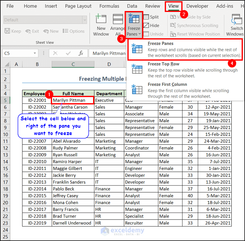
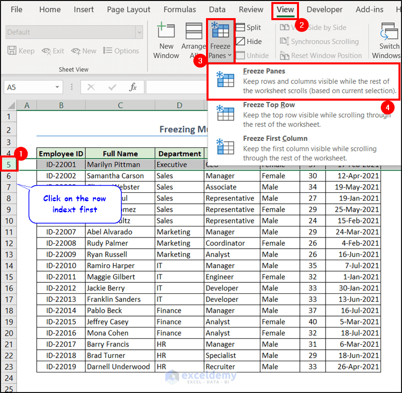
How To Freeze Panes In Excel - To instantaneously freeze the row and column. Excel freezes the first 3 rows. Go to the view tab and click the freeze panes button. You can also select row 4 and press the alt key > w > f > f. This guide will walk you through the process of freezing panes in excel, ensuring you can keep key information in view as you navigate through your spreadsheet. To remove freezing, follow these steps: To keep an area of a worksheet visible while you scroll to another area of the worksheet, go to the view tab, where you can freeze panes to lock specific rows and columns in place, or you can. Click on the view tab located in the ribbon, select the freeze panes dropdown, and select freeze first column from the dropdown menu. If you have a large table of data in excel, it can be useful to freeze rows or columns. Click on the “view” tab in the ribbon.

How To Freeze Panes Columns In Excel at Judith Tomlin blog

Click on the view tab located in the ribbon, select the freeze panes dropdown, and select freeze first column from the dropdown menu. This action will lock the first. This guide will walk you through the process of freezing panes in excel, ensuring you can keep key information in view as you navigate through your spreadsheet. To remove freezing, follow.

How to Freeze Panes in Excel YouTube

To remove freezing, follow these steps: You can also select row 4 and press the alt key > w > f > f. Select the cell below and to the right of the pane you want to freeze and click on the. Click on the view tab located in the ribbon, select the freeze panes dropdown, and select freeze first.

How to Freeze Selected Panes in Excel (4 Suitable Examples)

If you have a large table of data in excel, it can be useful to freeze rows or columns. This action will lock the first. This guide will walk you through the process of freezing panes in excel, ensuring you can keep key information in view as you navigate through your spreadsheet. To instantaneously freeze the row and column. Select.

How to Freeze Panes in Excel StepbyStep for PC and Mac

To instantaneously freeze the row and column. Click on ok and the freeze panes button will be available in the quick access toolbar. Select the row and the right of the column, then go to view select freeze panes. You can also select row 4 and press the alt key > w > f > f. Click the freeze panes.

How to Freeze Selected Panes in Excel (4 Suitable Examples)

Go to the view tab and click the freeze panes button. Click on ok and the freeze panes button will be available in the quick access toolbar. Click on the view tab located in the ribbon, select the freeze panes dropdown, and select freeze first column from the dropdown menu. Select the row and the right of the column, then.

How to Freeze Multiple Rows and Columns in Excel using Freeze Panes

Click the freeze panes option. This way you can keep rows or columns visible while scrolling through the rest of the worksheet. If you have a large table of data in excel, it can be useful to freeze rows or columns. Go to the view tab and click the freeze panes button. To remove freezing, follow these steps:

How to Freeze Panes in Excel Sheetaki

To instantaneously freeze the row and column. This way you can keep rows or columns visible while scrolling through the rest of the worksheet. Click on the “view” tab in the ribbon. From the drop down menu select if you want the header row, the first row of data, or the header column, the first column of data to be..

How To Freeze Panes Columns In Excel at Judith Tomlin blog

To remove freezing, follow these steps: In the “window” group, click the “freeze panes” dropdown and select unfreeze panes. This action will lock the first. Click the freeze panes option. When you freeze columns or rows, they are referred to as panes. this wikihow will show you how to freeze and unfreeze panes to lock rows and columns in excel.

How to Freeze and Unfreeze Panes in Excel (StepbyStep)

You can also select row 4 and press the alt key > w > f > f. This guide will walk you through the process of freezing panes in excel, ensuring you can keep key information in view as you navigate through your spreadsheet. If you have a large table of data in excel, it can be useful to freeze.

How to freeze Columns and Rows in Excel Using Freeze Panes Tool YouTube

Select the row and the right of the column, then go to view select freeze panes. To instantaneously freeze the row and column. From the drop down menu select if you want the header row, the first row of data, or the header column, the first column of data to be. Select the cell below and to the right of.