How To Make Negative Numbers Red In Excel
How To Make Negative Numbers Red In Excel - In this tutorial, you'll learn how to make negative numbers red in excel. We’re using conditional formatting and a couple of. This post is going to show you all the different ways you can use to display your negative numbers with red font color in microsoft excel. You can display negative numbers by using the minus sign, parentheses, or by applying a red color (with or without parentheses). Excel is great for organizing and analyzing data. By using simple conditional formatting techniques, you can. Under the home tab, click on conditional formatting > highlight cells rules > less than. In the less than dialog box, please configure as follows. Select the cell or range of cells that you want to format. Learn how to make negative numbers red with simple formatting tips for clearer data analysis. Make negative numbers stand out in excel! But sometimes, the default formatting isn't enough. Learn how to make negative numbers red with simple formatting tips for clearer data analysis. This post is going to show you all the different ways you can use to display your negative numbers with red font color in microsoft excel. Show negative numbers as red. But sometimes, the default formatting isn't enough. We have 3 quick and easy ways for you today to have the negative numbers in your spreadsheets displayed in red. We’re using conditional formatting and a couple of. You can use conditional formatting or a custom number formatting to do this. Excel is great for organizing and analyzing data. By using simple conditional formatting techniques, you can. In this article, i’ll show you how to easily show negative number as red in excel, which can make your data analysis much clearer. 4 easy ways to make negative numbers red in excel. Learn how to make negative numbers red with simple formatting tips for clearer data analysis. In the less. In this tutorial, you'll learn how to make negative numbers red in excel. You can display negative numbers by using the minus sign, parentheses, or by applying a red color (with or without parentheses). By using simple conditional formatting techniques, you can. But sometimes, the default formatting isn't enough. Make negative numbers stand out in excel! You can use conditional formatting or a custom number formatting to do this. Under the home tab, click on conditional formatting > highlight cells rules > less than. But sometimes, the default formatting isn't enough. We’re using conditional formatting and a couple of. In the less than dialog box, please configure as follows. Under the home tab, click on conditional formatting > highlight cells rules > less than. We have 3 quick and easy ways for you today to have the negative numbers in your spreadsheets displayed in red. This post is going to show you all the different ways you can use to display your negative numbers with red font color in. Say you have the list of numbers below in column b and want to. You can use conditional formatting or a custom number formatting to do this. In this article, i’ll show you how to easily show negative number as red in excel, which can make your data analysis much clearer. This post is going to show you all the. In this tutorial, you will learn how to format negative numbers with red font in excel and google sheets. Download the practice workbook and modify the data to find new results. Excel is great for organizing and analyzing data. Show negative numbers as red using. You can display negative numbers by using the minus sign, parentheses, or by applying a. Say you have the list of numbers below in column b and want to. This post is going to show you all the different ways you can use to display your negative numbers with red font color in microsoft excel. Show negative numbers as red using. 4 easy ways to make negative numbers red in excel. In this tutorial, you. Show negative numbers as red using. In this article, i’ll show you how to easily show negative number as red in excel, which can make your data analysis much clearer. Learn how to make negative numbers red with simple formatting tips for clearer data analysis. 4 easy ways to make negative numbers red in excel. Excel is great for organizing.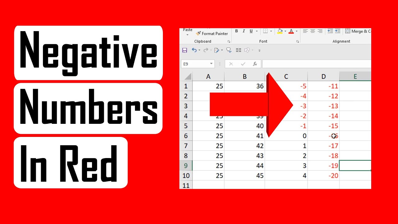
How To Highlight All Negative Numbers In Red In Excel YouTube

How to Make Negative Numbers Red in Excel Earn & Excel
Basic Excel Tutorial

How to Make Negative Numbers Red in Excel

How to Make Negative Numbers Red in Excel

How to Make Negative Accounting Numbers Red in Excel (3 Ways)

How to Make Negative Numbers Red in Excel
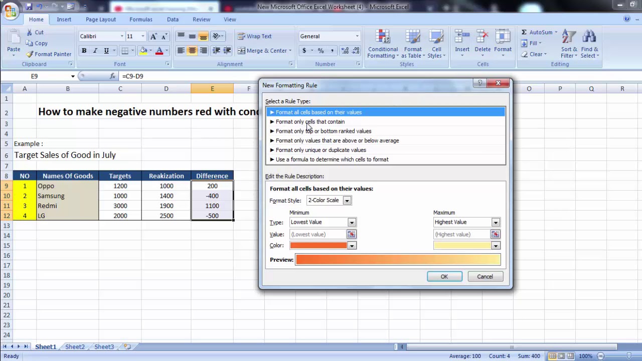
How to Create negative numbers red with conditional formatting in
![How to Make Negative Numbers Red in Excel? [With Examples]](http://officedigests.com/wp-content/uploads/2023/09/highlight-negative-numbers-in-red-number-formatting.jpg)
How to Make Negative Numbers Red in Excel? [With Examples]

How to Make Negative Numbers Red in Excel (4 Easy Ways)
Related Post: