How To Freeze Top Row In Excel
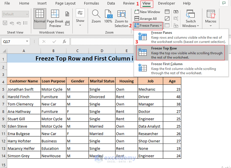
How To Freeze Top Row In Excel - Also, check to verify that at least one printer is set up in windows. When you do this, the border under row 1 is a little darker than other borders, meaning that the row above it is frozen. In the table properties dialog box, on the row tab, select the repeat as header row at the top of. For more information, such as freezing selected rows and columns in your workbook, see freeze panes. By splitting the worksheet, you can scroll down in the lower pane and still see the top rows in the upper pane. If you scroll down your worksheet but always see the same top rows, they're locked in place (frozen). If you want the row and column headers always visible when you scroll through your worksheet, you can lock the top row and/or first column. If the print titles ribbon button is grayed out, check to ensure that you’re not currently editing a cell or an area chart. Select the cell below the rows, and to the right of the columns you want to freeze. Tap view > freeze panes, and then tap the. For more information, such as freezing selected rows and columns in your workbook, see freeze panes. Also, check to verify that at least one printer is set up in windows. For example, select cell b3 if you want to freeze the first two rows and the first column. Select the cell below the rows, and to the right of the. When you do this, the border under row 1 is a little darker than other borders, meaning that the row above it is frozen. Use the unfreeze panes command to unlock those rows. If you want the row and column headers always visible when you scroll through your worksheet, you can lock the top row and/or first column. Tap view. When you do this, the border under row 1 is a little darker than other borders, meaning that the row above it is frozen. Select the cell below the rows, and to the right of the columns you want to freeze. Tap view > freeze panes, and then tap the. How to freeze panes in excel to keep rows or. For example, select cell b3 if you want to freeze the first two rows and the first column. To split this worksheet as shown above, you select below the row where you want. How to freeze panes in excel to keep rows or columns in your worksheet visible while you scroll, or lock them in place to create multiple worksheet. For example, select cell b3 if you want to freeze the first two rows and the first column. How to freeze panes in excel to keep rows or columns in your worksheet visible while you scroll, or lock them in place to create multiple worksheet areas. When you do this, the border under row 1 is a little darker than. Select the cell below the rows, and to the right of the columns you want to freeze. Also, check to verify that at least one printer is set up in windows. Tap view > freeze panes, and then tap the. By splitting the worksheet, you can scroll down in the lower pane and still see the top rows in the. In the columns to repeat at left box, enter the reference of the columns that contain the row labels. Select view, select freeze panes, then select freeze top row. By splitting the worksheet, you can scroll down in the lower pane and still see the top rows in the upper pane. For more information, such as freezing selected rows and. For more information, such as freezing selected rows and columns in your workbook, see freeze panes. If you scroll down your worksheet but always see the same top rows, they're locked in place (frozen). To split this worksheet as shown above, you select below the row where you want. If the print titles ribbon button is grayed out, check to. In the columns to repeat at left box, enter the reference of the columns that contain the row labels. How to freeze panes in excel to keep rows or columns in your worksheet visible while you scroll, or lock them in place to create multiple worksheet areas. Use the unfreeze panes command to unlock those rows. Select view, select freeze. When you do this, the border under row 1 is a little darker than other borders, meaning that the row above it is frozen. In the table properties dialog box, on the row tab, select the repeat as header row at the top of. If the print titles ribbon button is grayed out, check to ensure that you’re not currently.
How To Freeze Top Row In Excel (Easy Guide) ExcelTutorial
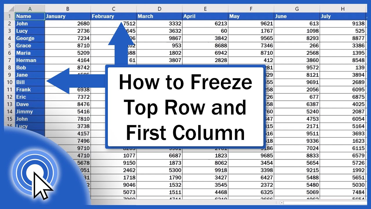
How to Freeze Top Row and First Column in Excel (Quick and Easy) YouTube

How To Freeze Top Row In Excel (Easy Guide) ExcelTutorial
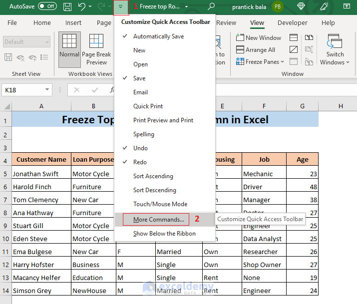
How to Freeze Top Row and First Column in Excel (5 Methods)
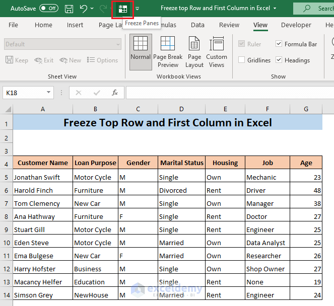
How to Freeze Top Row and First Column in Excel (5 Methods)

How to Freeze/Unfreeze Panes in Excel
How to Freeze Top Row and First Column in Excel (5 Methods)

How to Freeze Panes in Excel A Beginner's Guide

How To Freeze Rows In Excel

How To Freeze Top Row In Excel (Easy Guide) ExcelTutorial
Related Post: