How To Freeze Selected Rows In Excel

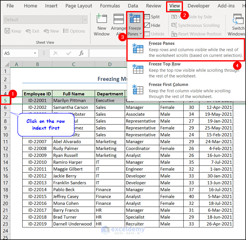
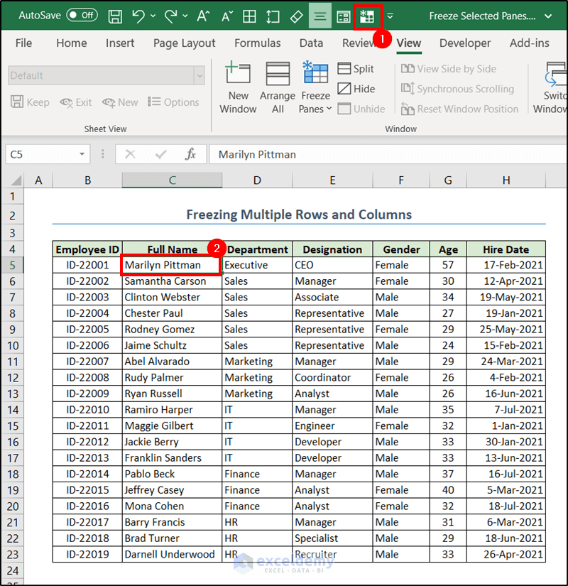
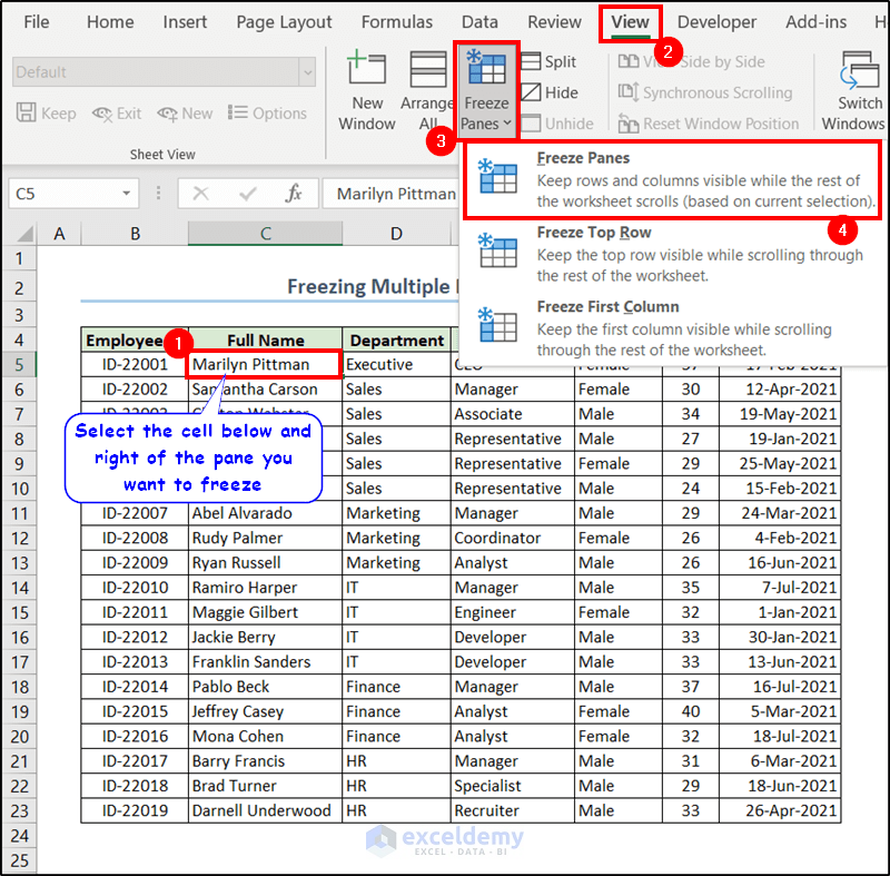
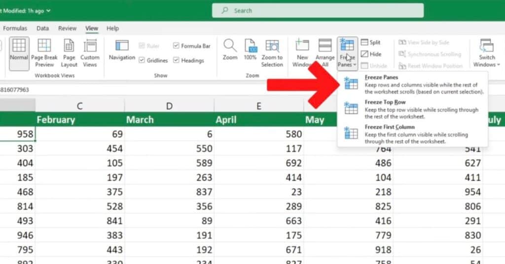
How To Freeze Selected Rows In Excel - Make sure your data is already organized in. Then, go to the “view” tab, click “freeze. Click the view tab on the excel ribbon located at the top. Select the cell that is just to the right and to the bottom of the rows and. Here’s how to do it: Freezing rows or columns in excel ensures that certain cells remain visible as you scroll through the data. Freezing the top row is the most common use of this feature, as the first row usually contains the headers. To keep an area of a worksheet visible while you scroll to another area of the worksheet, go to the view tab, where you can freeze panes to lock specific rows and columns in place, or you can. Use this method to lock multiple rows or columns at the same time or to lock rows and columns at the same time. If you want to easily edit two parts of the spreadsheet at once, splitting.

How to freeze multiple rows in excel 2025 Freeze panes to lock rows

Freezing rows or columns in excel ensures that certain cells remain visible as you scroll through the data. Then navigate to the window group of command icons and select the freeze panes command. You can freeze one or more rows in an excel worksheet using the freeze panes command. Select the fifth row (the row after the freezing should end).

How To Freeze Multiple Rows in Excel

Click the view tab on the excel ribbon located at the top. You can freeze one or more rows in an excel worksheet using the freeze panes command. To keep an area of a worksheet visible while you scroll to another area of the worksheet, go to the view tab, where you can freeze panes to lock specific rows and.

How to Freeze Multiple Rows and Columns in Excel using Freeze Panes

This way you can keep rows or columns visible while scrolling through the rest of the worksheet. If you have a large table of data in excel, it can be useful to freeze rows or columns. Freezing rows or columns in excel ensures that certain cells remain visible as you scroll through the data. Click the view tab on the.

How to Freeze Multiple Rows and or Columns in Excel using Freeze Panes

Select the fifth row (the row after the freezing should end) by clicking on the row index on the left of the spreadsheet. Freezing rows or columns in excel ensures that certain cells remain visible as you scroll through the data. Click the view tab on the excel ribbon located at the top. Here’s how to do it: If you.

How to Freeze Selected Panes in Excel (4 Suitable Examples)

If you want to easily edit two parts of the spreadsheet at once, splitting. If you have a large table of data in excel, it can be useful to freeze rows or columns. To freeze your selected row, click on “freeze panes.” freezing panes is straightforward, but here are some additional tips to help you use this feature more effectively..

How to Freeze Selected Panes in Excel (4 Suitable Examples)

Here’s how to do it: You can freeze one or more rows in an excel worksheet using the freeze panes command. If you want to easily edit two parts of the spreadsheet at once, splitting. Freezing the top row is the most common use of this feature, as the first row usually contains the headers. Click the view tab on.

How to Freeze Multiple Rows and Columns in Excel using Freeze Panes

Go to the view tab and select freeze panes from the. If you have a large table of data in excel, it can be useful to freeze rows or columns. Here’s how to do it: Select the fifth row (the row after the freezing should end) by clicking on the row index on the left of the spreadsheet. Use this.

How to Freeze Multiple Rows and or Columns in Excel using Freeze Panes

If you have a large table of data in excel, it can be useful to freeze rows or columns. Freezing the top row is the most common use of this feature, as the first row usually contains the headers. Freezing rows or columns in excel ensures that certain cells remain visible as you scroll through the data. To freeze your.

How to Freeze Selected Panes in Excel (4 Suitable Examples)

Then navigate to the window group of command icons and select the freeze panes command. Yes, you can freeze multiple rows and columns by selecting the cell below and to the right of the rows and columns you want to freeze. Freezing rows or columns in excel ensures that certain cells remain visible as you scroll through the data. Make.

How to Freeze Rows in Excel Beginner's Guide Sheet Leveller

Freezing the top row is the most common use of this feature, as the first row usually contains the headers. You can freeze one or more rows in an excel worksheet using the freeze panes command. Go to the view tab and select freeze panes from the. Then, go to the “view” tab, click “freeze. If you freeze rows containing.