How To Freeze Multiple Rows In Excel

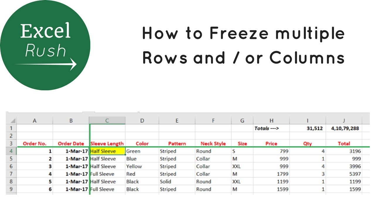
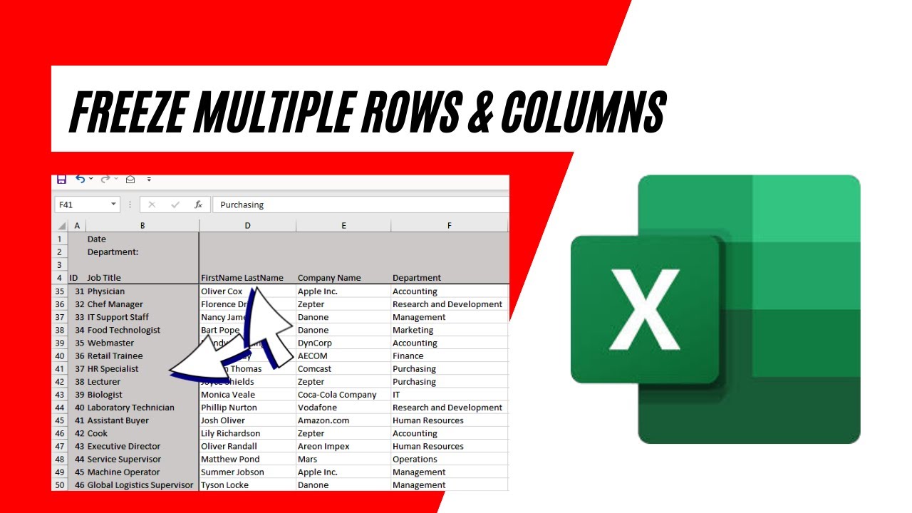
How To Freeze Multiple Rows In Excel - In this guide, i’ll show you how to freeze multiple rows in excel using every method possible. We want to freeze rows 1 to 9 in our case, so we chose row 10. In your spreadsheet, select the row below the rows that you want to freeze. Select the cell that is just to the right and to the bottom of the rows and. To freeze rows, execute the following steps. To freeze both rows and columns, click on the cell that is immediately below the rows you want to freeze and immediately to the right of the columns you want to freeze. You can freeze one or more rows in an excel worksheet using the freeze panes command. Keep key data in view while scrolling through your spreadsheet seamlessly. To keep an area of a worksheet visible while you scroll to another area of the worksheet, go to the view tab, where you can freeze panes to lock specific rows and columns in place, or you can. On the view tab, in the window group, click freeze panes.

How to Freeze Multiple Rows and Columns in Excel using Freeze Panes

In your spreadsheet, select the row below the rows that you want to freeze. On the view tab, in the window group, click freeze panes. If you freeze rows containing headings, the headings will appear when you scroll. In this article, i’ll guide you through the steps on how to freeze. Select the cell that is just to the right.

How to Freeze Multiple Rows and or Columns in Excel using Freeze Panes

Use this method to lock multiple rows or columns at the same time or to lock rows and columns at the same time. To freeze both rows and columns, click on the cell that is immediately below the rows you want to freeze and immediately to the right of the columns you want to freeze. You can freeze one or.

How to Freeze Multiple Rows or Columns in Excel using Freeze Panes

On the view tab, in the window group, click freeze panes. For example, if you want to freeze the first three rows, select the fourth row. To freeze both rows and columns, click on the cell that is immediately below the rows you want to freeze and immediately to the right of the columns you want to freeze. In this.

How to Freeze Multiple Rows and or Columns in Excel using Freeze Panes

For example, select row 4. To freeze rows, execute the following steps. If you freeze rows containing headings, the headings will appear when you scroll. Freezing rows in excel is a simple yet powerful feature that ensures your key data stays visible, no matter how far you scroll. To freeze both rows and columns, click on the cell that is.

How To Freeze Multiple Rows in Excel

Scroll down to the rest of the. For example, if you want to freeze the first three rows, select the fourth row. To keep an area of a worksheet visible while you scroll to another area of the worksheet, go to the view tab, where you can freeze panes to lock specific rows and columns in place, or you can..

How to freeze multiple rows and or columns in excel 2023 tutorial river

In your spreadsheet, select the row below the rows that you want to freeze. For example, select row 4. Keep key data in view while scrolling through your spreadsheet seamlessly. In this guide, i’ll show you how to freeze multiple rows in excel using every method possible. For example, if you want to freeze the first three rows, select the.

How to Freeze Multiple Rows and Columns in Excel YouTube

To freeze both rows and columns, click on the cell that is immediately below the rows you want to freeze and immediately to the right of the columns you want to freeze. To freeze rows, execute the following steps. In this article, i’ll guide you through the steps on how to freeze. On the view tab, in the window group,.

How to Freeze Multiple Rows and Columns in Excel Using Freeze Panes

To keep an area of a worksheet visible while you scroll to another area of the worksheet, go to the view tab, where you can freeze panes to lock specific rows and columns in place, or you can. Freezing rows in excel is a simple yet powerful feature that ensures your key data stays visible, no matter how far you.

How to Freeze Multiple Rows in Excel (Quick and Easy) YouTube

If you freeze rows containing headings, the headings will appear when you scroll. On the view tab, in the window group, click freeze panes. Freezing rows in excel is a simple yet powerful feature that ensures your key data stays visible, no matter how far you scroll. For example, select row 4. To freeze both rows and columns, click on.

How to freeze multiple rows in excel 2025 Freeze panes to lock rows

For example, if you want to freeze the first three rows, select the fourth row. In this article, i’ll guide you through the steps on how to freeze. Use this method to lock multiple rows or columns at the same time or to lock rows and columns at the same time. Keep key data in view while scrolling through your.