Excel Pivot Hide Grand Total
Excel Pivot Hide Grand Total - The dollar sign allows you to fix either the row, the column or both on any cell reference, by preceding the column or row with the dollar sign. It would mean you can apply textual functions like left/right/mid on a conditional basis without. As far as i can tell, excel xp (which is what we're using). How can i declare the following if condition properly? We use syncfusions essential xlsio to output values to an excel document which works great. To solve this problem in excel, usually i would just type in the literal row number of the cell above, e.g., if i'm typing in cell a7, i would use the formula =a6. Boolean values true and false in excel are treated as 1 and 0, but we need to convert them. But i can't figure out. In a text about excel i have read the following: I am trying to use the if function to assign a value to a cell depending on another cells value so, if the value in column 'e' is 1, then the value in column g should be the same. But i can't figure out. I am trying to use the if function to assign a value to a cell depending on another cells value so, if the value in column 'e' is 1, then the value in column g should be the same. The dollar sign allows you to fix either the row, the column or both on any. If a1 = n/a then c1 = b1 else if a1 != n/a or has value(int) then c1 = a1*b1 The dollar sign allows you to fix either the row, the column or both on any cell reference, by preceding the column or row with the dollar sign. To convert them into numbers 1 or 0, do some mathematical operation.. =sum(!b1:!k1) when defining a name for a cell and this was entered into the refers to field. Boolean values true and false in excel are treated as 1 and 0, but we need to convert them. We use syncfusions essential xlsio to output values to an excel document which works great. What is the best way of representing a datetime. =sum(!b1:!k1) when defining a name for a cell and this was entered into the refers to field. Now excel will calculate regressions using both x 1 and x 2 at the same time: The dollar sign allows you to fix either the row, the column or both on any cell reference, by preceding the column or row with the dollar. I am trying to use the if function to assign a value to a cell depending on another cells value so, if the value in column 'e' is 1, then the value in column g should be the same. =sum(!b1:!k1) when defining a name for a cell and this was entered into the refers to field. To solve this problem. We use syncfusions essential xlsio to output values to an excel document which works great. I need help on my excel sheet. As far as i can tell, excel xp (which is what we're using). How to actually do it the impossibly tricky part there's no obvious way to see the other regression. But i can't figure out. The dollar sign allows you to fix either the row, the column or both on any cell reference, by preceding the column or row with the dollar sign. In a text about excel i have read the following: In your example you fix the column to b and. I need to parse an iso8601 date/time format with an included timezone. To convert them into numbers 1 or 0, do some mathematical operation. I am trying to use the if function to assign a value to a cell depending on another cells value so, if the value in column 'e' is 1, then the value in column g should be the same. How to actually do it the impossibly tricky part. I need help on my excel sheet. If a1 = n/a then c1 = b1 else if a1 != n/a or has value(int) then c1 = a1*b1 Then if i copied that. We use syncfusions essential xlsio to output values to an excel document which works great. =sum(!b1:!k1) when defining a name for a cell and this was entered into. How can i declare the following if condition properly? In a text about excel i have read the following: =sum(!b1:!k1) when defining a name for a cell and this was entered into the refers to field. Now excel will calculate regressions using both x 1 and x 2 at the same time: I am trying to use the if function.
MS Excel 2010 How to Remove Row Grand Totals in a Pivot Table
How To Hide 0 Grand Total In Pivot Table
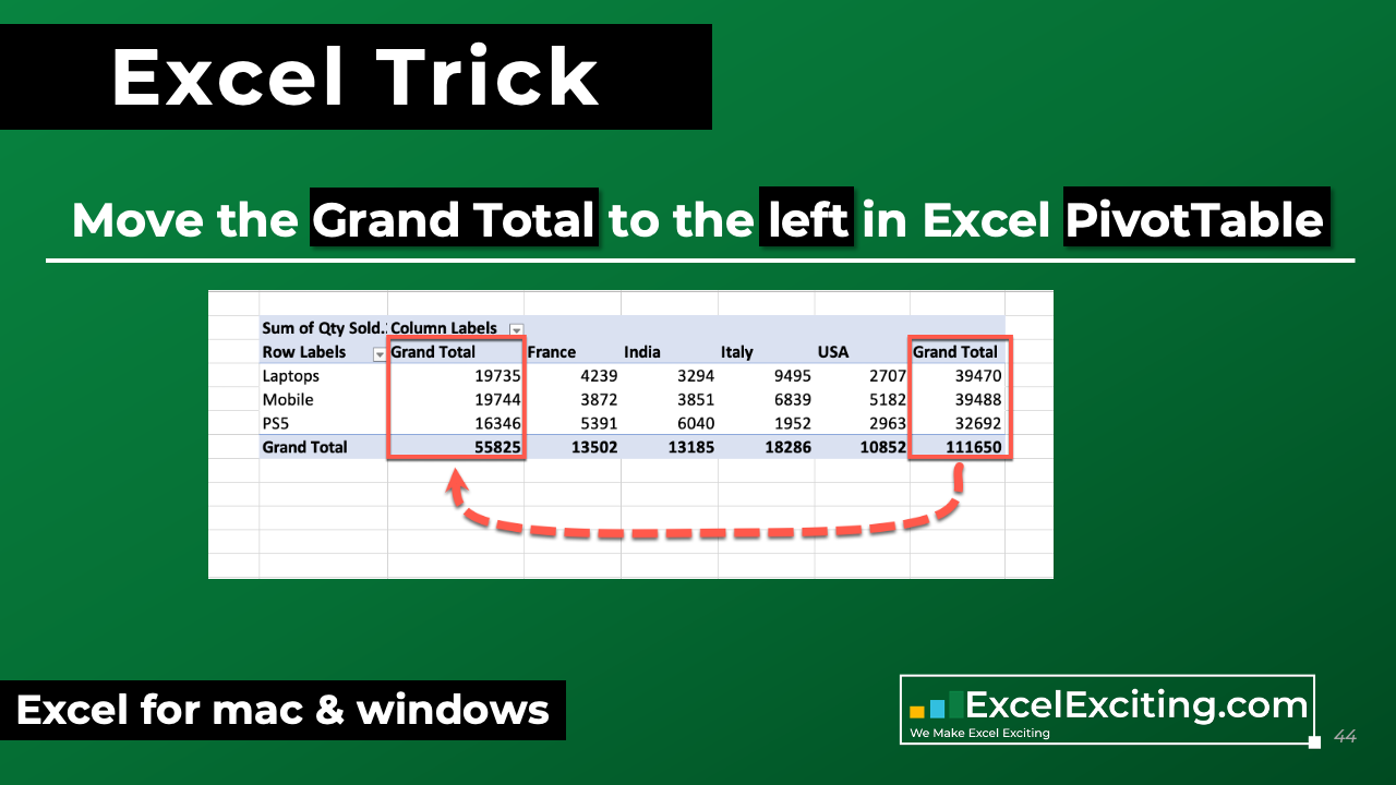
How To Move Grand Total Row In Pivot Table To Top Printable Online
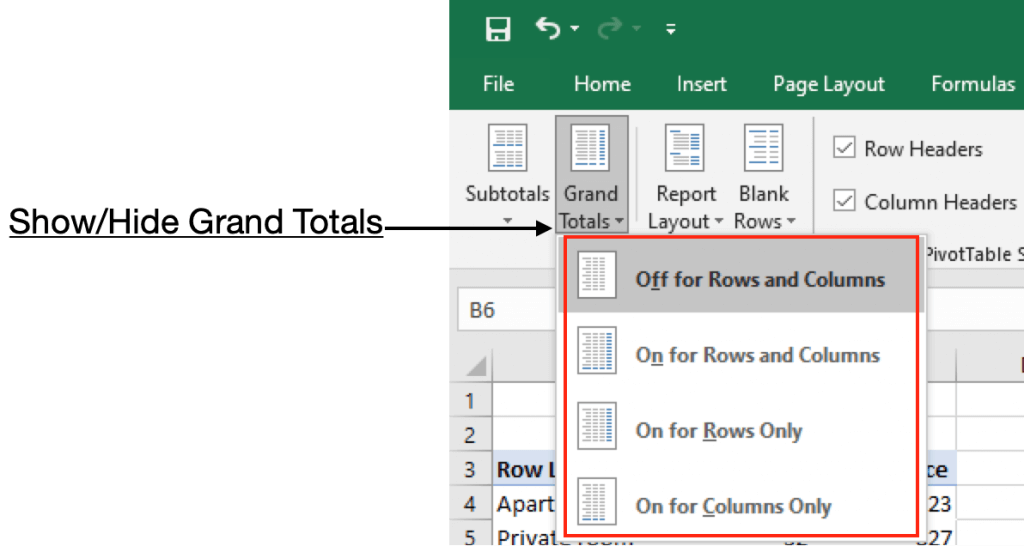
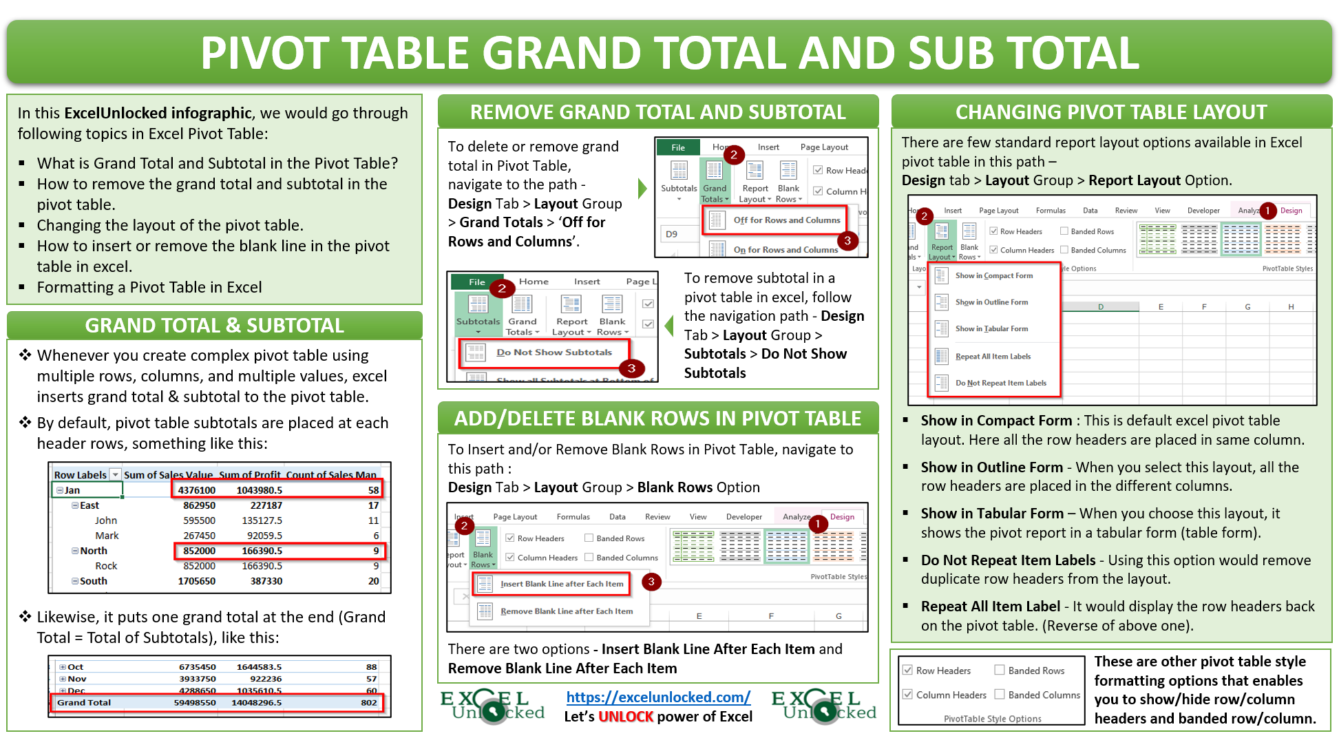
How to Show/Hide Grand totals in Pivot Table Excel
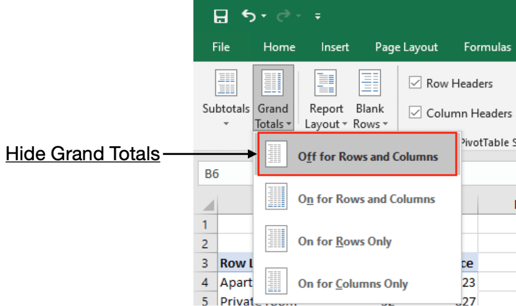
How to Show/Hide Grand totals in Pivot Table Excel

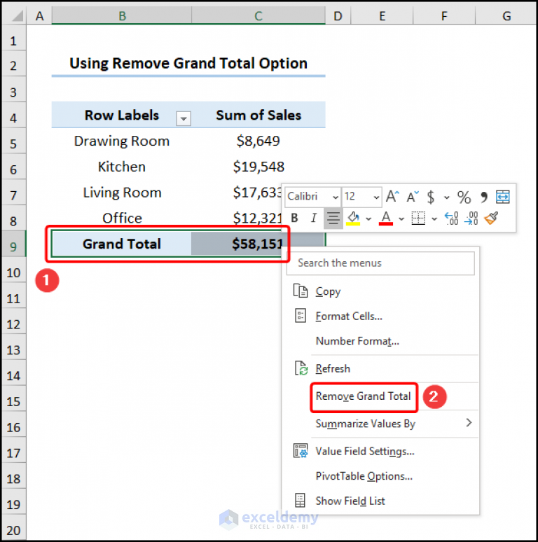
How to Remove Grand Total in a Pivot Table

Remove Grand Total From Pivot Table in Excel (Easy Steps)

Remove Grand Total From Pivot Table in Excel (Easy Steps)

Excel How to Remove Grand Total from Pivot Table
How to Remove Grand Total from Pivot Table (4 Quick Ways)
Related Post: