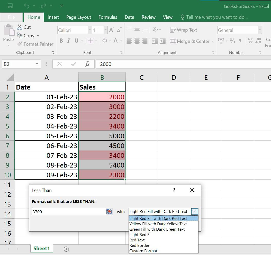
Excel Conditional Format
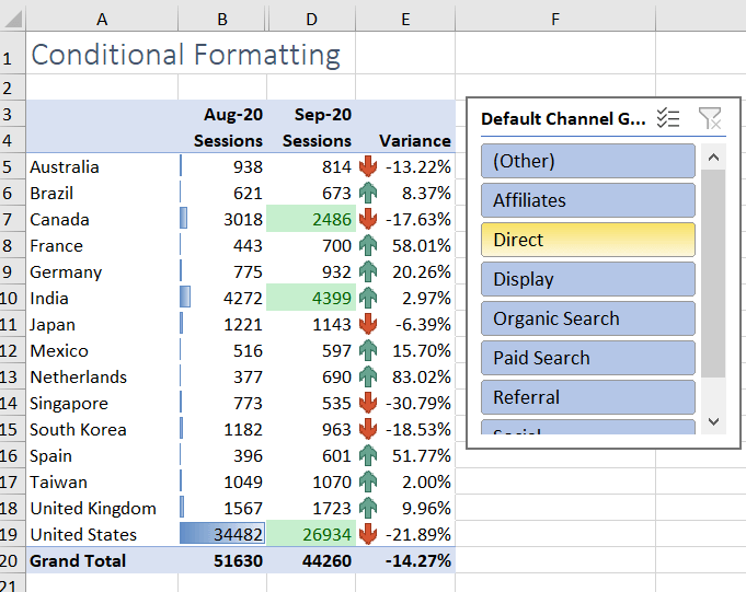
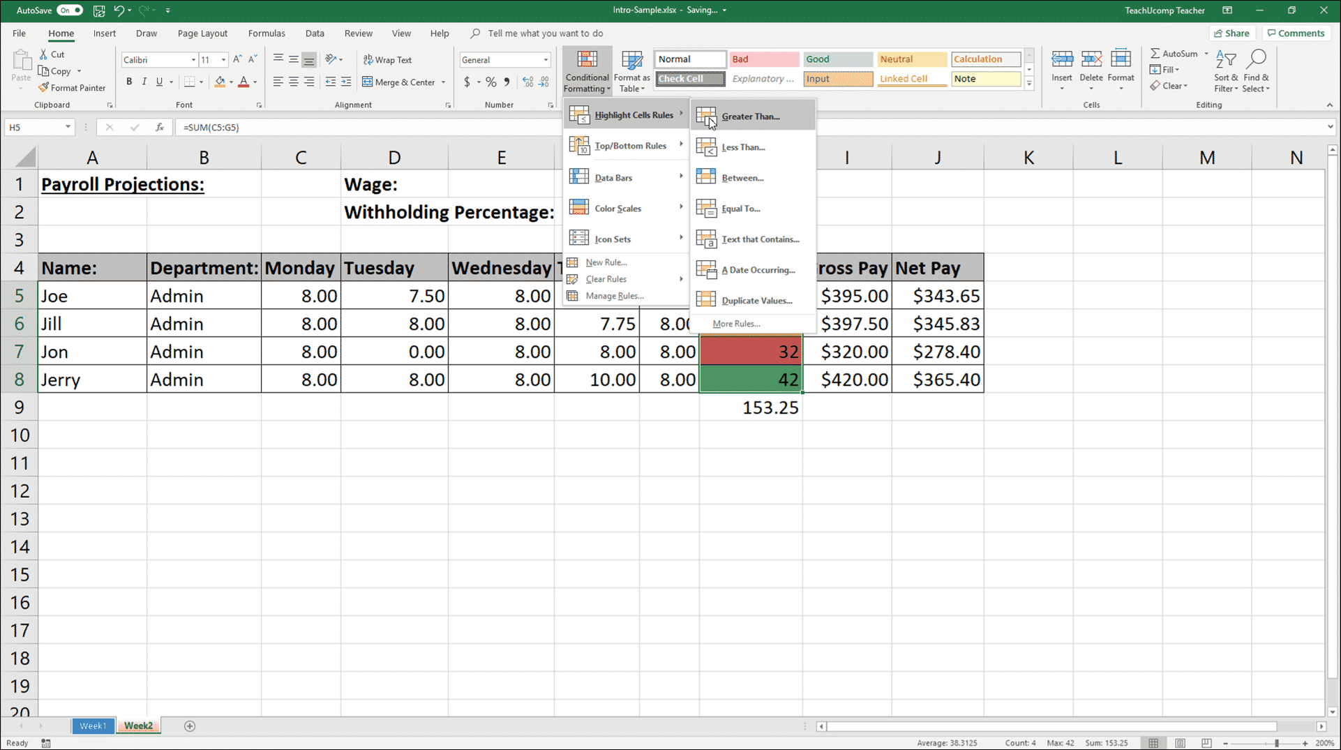
Excel Conditional Format - Select the cells you want to check for. Use conditional formatting to find and highlight duplicate data. You can use conditional formatting to highlight cells that contain values that meet a certain condition, or format a whole cell range and vary the exact format as the value of each cell varies. There are several ways to hide error values and error. Follow these steps to create a custom formatting rule—which will only be available in the worksheet in which you create it. In excel, from the home tab, click conditional formatting > new rule. For example, format blank cells, or see which salespeople are selling above average, or track who. Next, select the “ use a formula to determine which cells to format ” option, enter your formula and apply the format of. That way you can review the duplicates and decide if you want to remove them. In a worksheet, select the range of cells in which you’ll be. Use conditional formatting to find and highlight duplicate data. This rule uses a formula to determine whether a row is even or odd. That way you can review the duplicates and decide if you want to remove them. Testing whether conditions are true or false and making logical comparisons between expressions are common to many tasks. You can use conditional. Follow these steps to create a custom formatting rule—which will only be available in the worksheet in which you create it. For example, format blank cells, or see which salespeople are selling above average, or track who. Next, select the “ use a formula to determine which cells to format ” option, enter your formula and apply the format of.. In excel, from the home tab, click conditional formatting > new rule. When your formulas have errors that you anticipate and don't need to correct, but you want to improve the display of your results. For example, format blank cells, or see which salespeople are selling above average, or track who. How to use conditional formatting in excel to visually. To edit the conditional formatting rule, click one of the cells that has the rule applied, go to home > conditional formatting > manage rules > edit rule, and then make your changes. This rule uses a formula to determine whether a row is even or odd. When your formulas have errors that you anticipate and don't need to correct,. In a worksheet, select the range of cells in which you’ll be. When your formulas have errors that you anticipate and don't need to correct, but you want to improve the display of your results. You can use the and, or, not, and if functions to create. To edit the conditional formatting rule, click one of the cells that has. You can use conditional formatting to highlight cells that contain values that meet a certain condition, or format a whole cell range and vary the exact format as the value of each cell varies. Testing whether conditions are true or false and making logical comparisons between expressions are common to many tasks. There are several ways to hide error values. That way you can review the duplicates and decide if you want to remove them. This rule uses a formula to determine whether a row is even or odd. How to use conditional formatting in excel to visually explore, analyze, and identify patterns and trends. Select the cells you want to check for. Next, select the “ use a formula. You can use conditional formatting to highlight cells that contain values that meet a certain condition, or format a whole cell range and vary the exact format as the value of each cell varies. You can use the and, or, not, and if functions to create. How to use conditional formatting in excel to visually explore, analyze, and identify patterns. In a worksheet, select the range of cells in which you’ll be. Use conditional formatting to find and highlight duplicate data. There are several ways to hide error values and error. That way you can review the duplicates and decide if you want to remove them. For example, format blank cells, or see which salespeople are selling above average, or. You can use conditional formatting to highlight cells that contain values that meet a certain condition, or format a whole cell range and vary the exact format as the value of each cell varies. Next, select the “ use a formula to determine which cells to format ” option, enter your formula and apply the format of. Use conditional formatting.
Conditional Formatting in Excel The Complete Guide Layer Blog
Excel Conditional Formatting (with Examples)

Conditional Formatting Microsoft Excel
Conditional Formatting in Excel a Beginner's Guide
Conditional Formatting in Excel Instructions Inc.
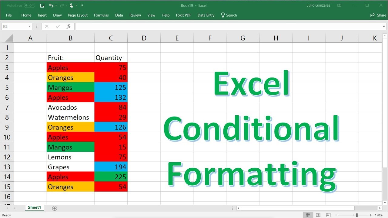
Excel Conditional Formatting Tutorial YouTube
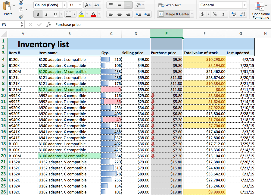
![Conditional Formatting in Excel [A HowTo Guide]](https://cdn.careerfoundry.com/en/wp-content/uploads/old-blog-uploads/equal-to.png)
Conditional Formatting in Excel [A HowTo Guide]

How to use Conditional Formatting in Excel?

Conditional Formatting in Excel
Excel Conditional Formatting HowTo Smartsheet
Related Post: