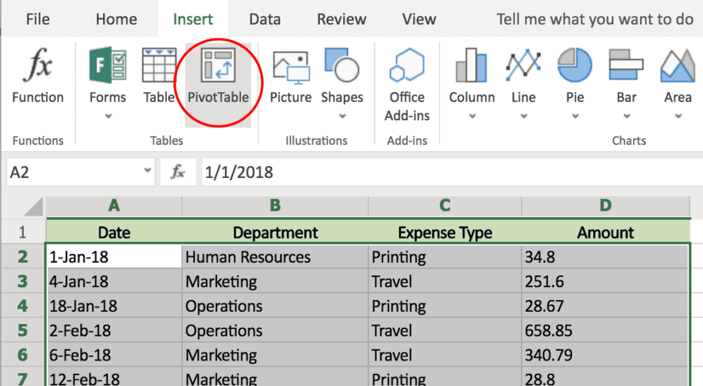
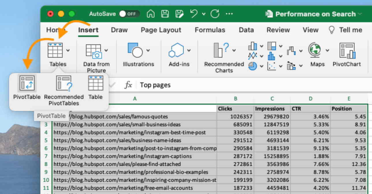
Creating Pivot Table In Excel
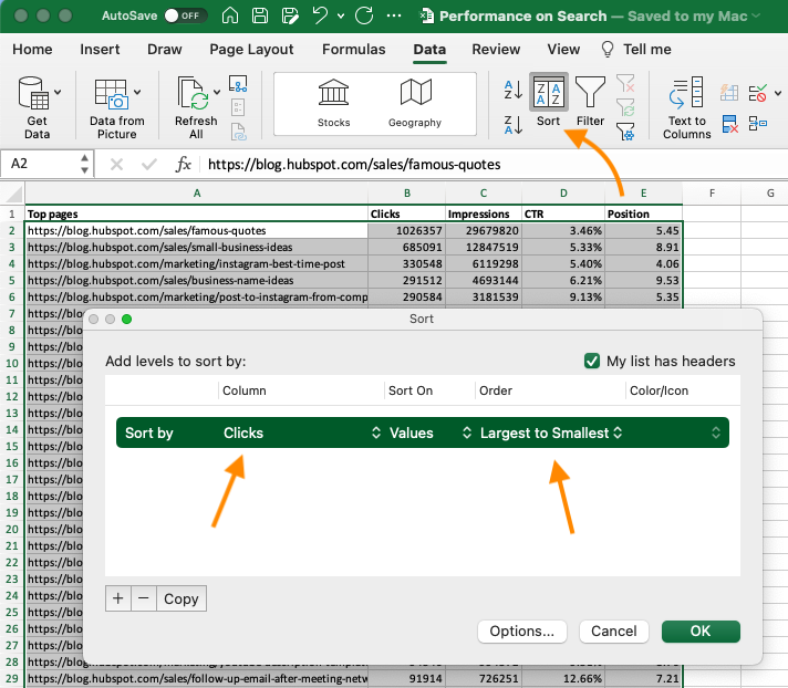
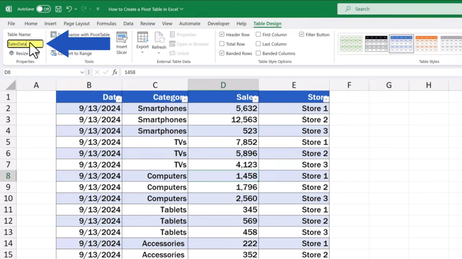
Creating Pivot Table In Excel - In the measure dialog box, for table name, click the down arrow, and then select the table you want the. In excel, show items or values in logical groups like months or quarters for ease of summarizing and performing data analysis. In the excel window, click power pivot> calculations> measures> new measure. In that case, you’ll connect to the external data source, and then create a pivottable to summarize, analyze, explore, and present that data. You can import related tables from databases, or set relationships in power pivot after you import. You might do this if you want to use power pivot. Build pivottables by using related tables in the field list. Excel will add some sample data to your worksheet, analyze it, then add recommended charts to the pane. If you want to sort or filter the columns of data. Follow the steps in the get started section to insert any of the recommended pivot. How to use a pivottable in excel to calculate, summarize, and analyze your worksheet data to see hidden patterns and trends. In the excel window, click power pivot> calculations> measures> new measure. In the measure dialog box, for table name, click the down arrow, and then select the table you want the. In that case, you’ll connect to the external. A model can contain a single table. Follow the steps in the get started section to insert any of the recommended pivot. How to use a pivottable in excel to calculate, summarize, and analyze your worksheet data to see hidden patterns and trends. Excel will add some sample data to your worksheet, analyze it, then add recommended charts to the. To create a model based on just one table, select the table and click add to data model in power pivot. Follow the steps in the get started section to insert any of the recommended pivot. A model can contain a single table. How to use a pivottable in excel to calculate, summarize, and analyze your worksheet data to see. After you create a pivottable, you'll see the field list. You might do this if you want to use power pivot. Follow the steps in the get started section to insert any of the recommended pivot. How to use a pivottable in excel to calculate, summarize, and analyze your worksheet data to see hidden patterns and trends. You can change. You might do this if you want to use power pivot. Build pivottables by using related tables in the field list. How to use a pivottable in excel to calculate, summarize, and analyze your worksheet data to see hidden patterns and trends. A model can contain a single table. In excel, show items or values in logical groups like months. Excel will add some sample data to your worksheet, analyze it, then add recommended charts to the pane. If you want to sort or filter the columns of data. A model can contain a single table. Here’s how to create a pivottable by. After you create a pivottable, you'll see the field list. In the excel window, click power pivot> calculations> measures> new measure. Follow the steps in the get started section to insert any of the recommended pivot. Excel will add some sample data to your worksheet, analyze it, then add recommended charts to the pane. After you create a pivottable, you'll see the field list. You can import related tables from. How to use a pivottable in excel to calculate, summarize, and analyze your worksheet data to see hidden patterns and trends. After you create a pivottable, you'll see the field list. Follow the steps in the get started section to insert any of the recommended pivot. Build pivottables by using related tables in the field list. A model can contain. You can import related tables from databases, or set relationships in power pivot after you import. A model can contain a single table. You might do this if you want to use power pivot. In the excel window, click power pivot> calculations> measures> new measure. If you want to sort or filter the columns of data. To create a model based on just one table, select the table and click add to data model in power pivot. In the measure dialog box, for table name, click the down arrow, and then select the table you want the. Here’s how to create a pivottable by. Create a pivotchart based on complex data that has text entries and.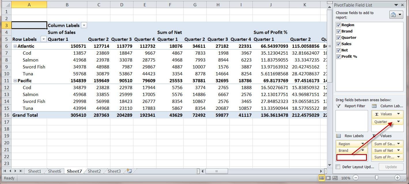
Top 3 Tutorials on Creating a Pivot Table in Excel

How to Create Pivot Tables in Microsoft Excel Quick Guide
How to Create a Pivot Table in Excel A Comprehensive Guide to the
How to Create a Pivot Table in Excel (A Comprehensive Guide for
How to create Pivot Tables in Excel Nexacu

How To Create A Pivot Table How To Excel PELAJARAN
How to Create a Pivot Table in Excel A StepbyStep Tutorial
How To Create A Pivot Table From Different Sheets In Excel Templates

3 Easy Ways to Create Pivot Tables in Excel (with Pictures)

How To Create a Pivot Table in Excel
Related Post: