Create Pie Charts In Excel
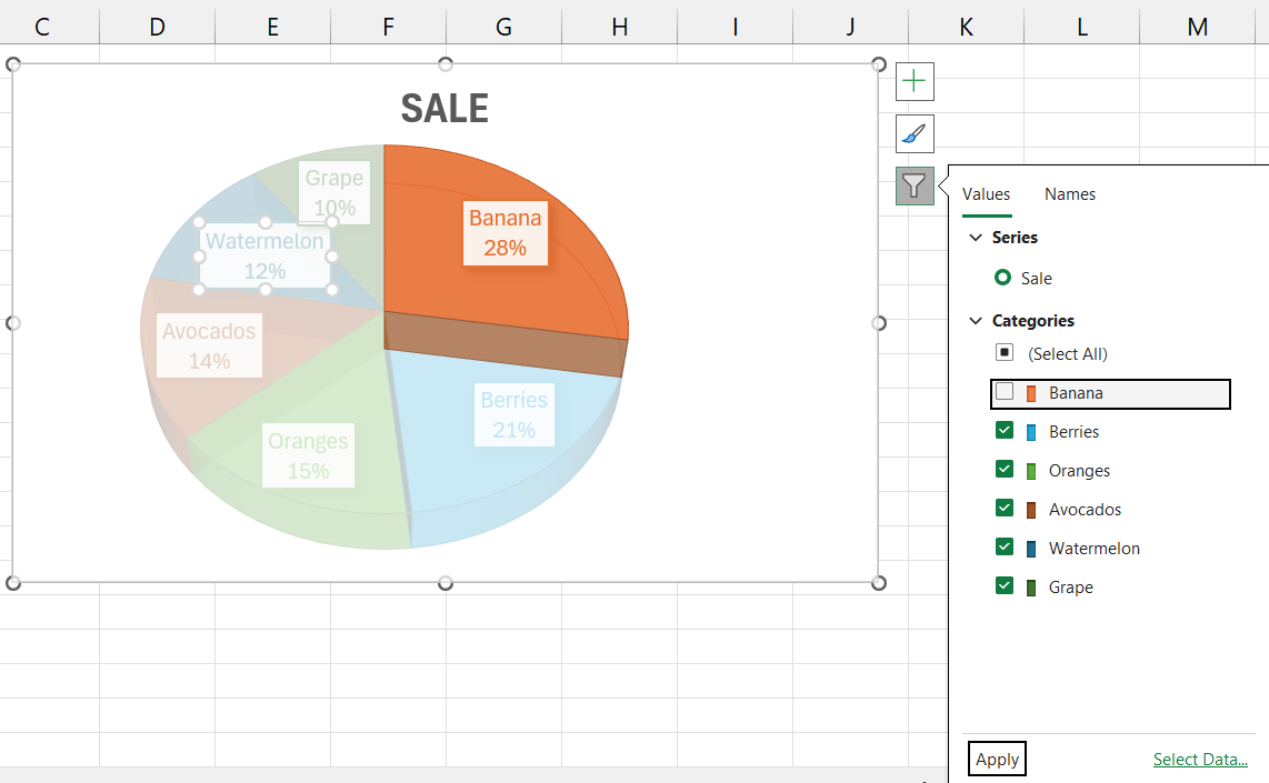
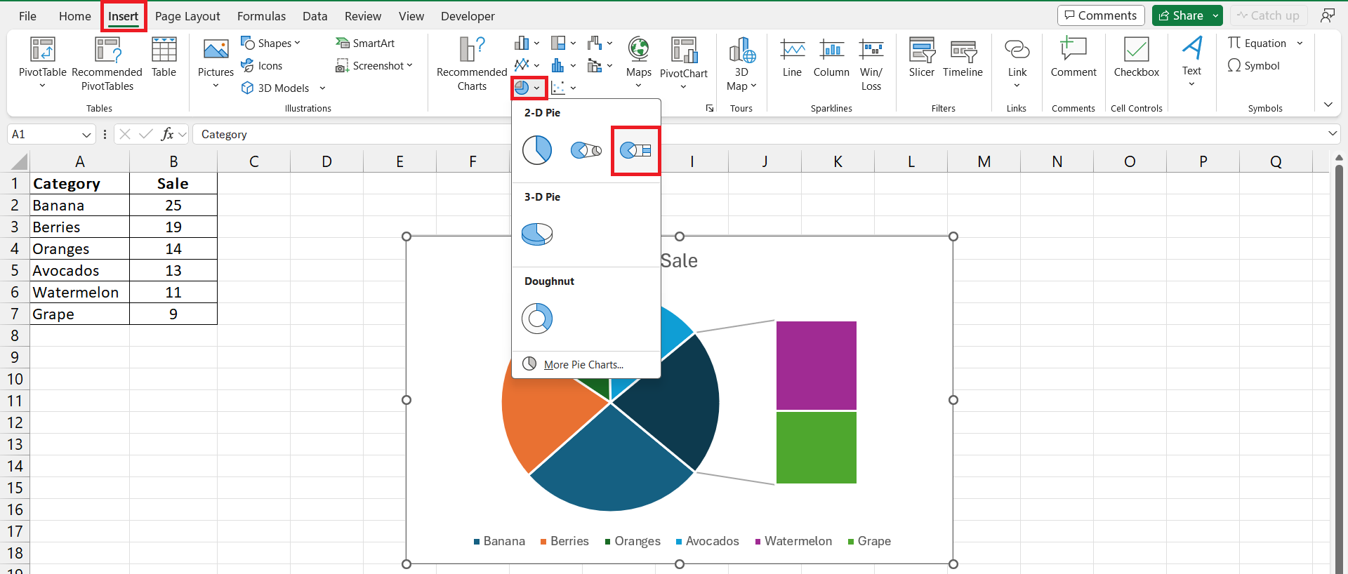
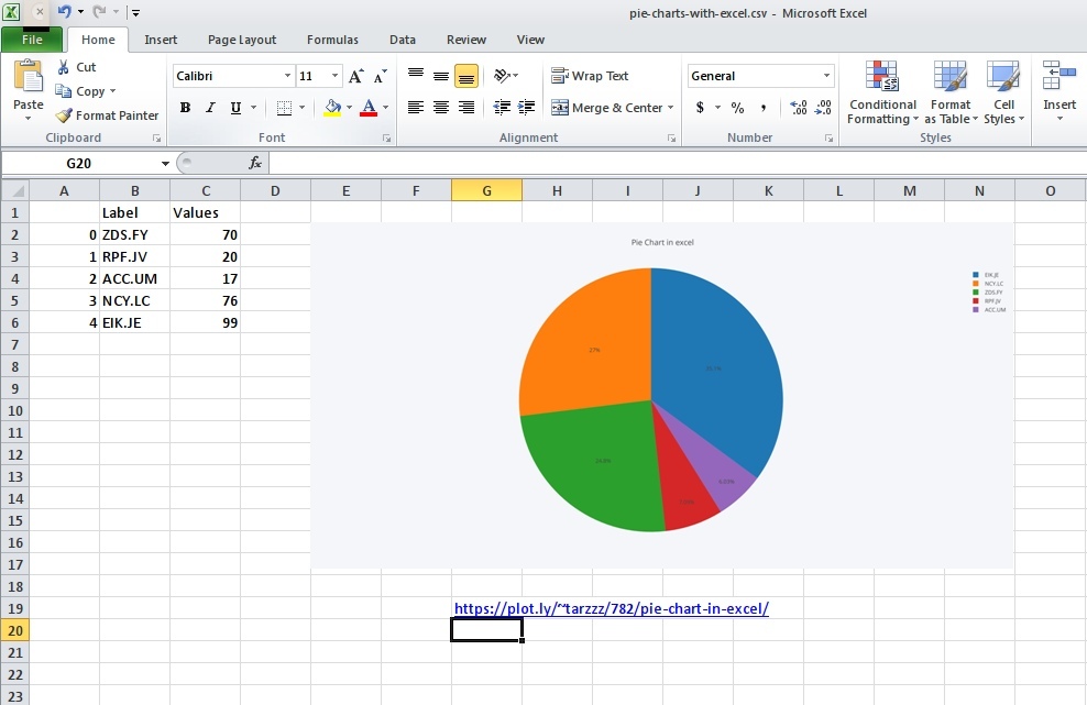
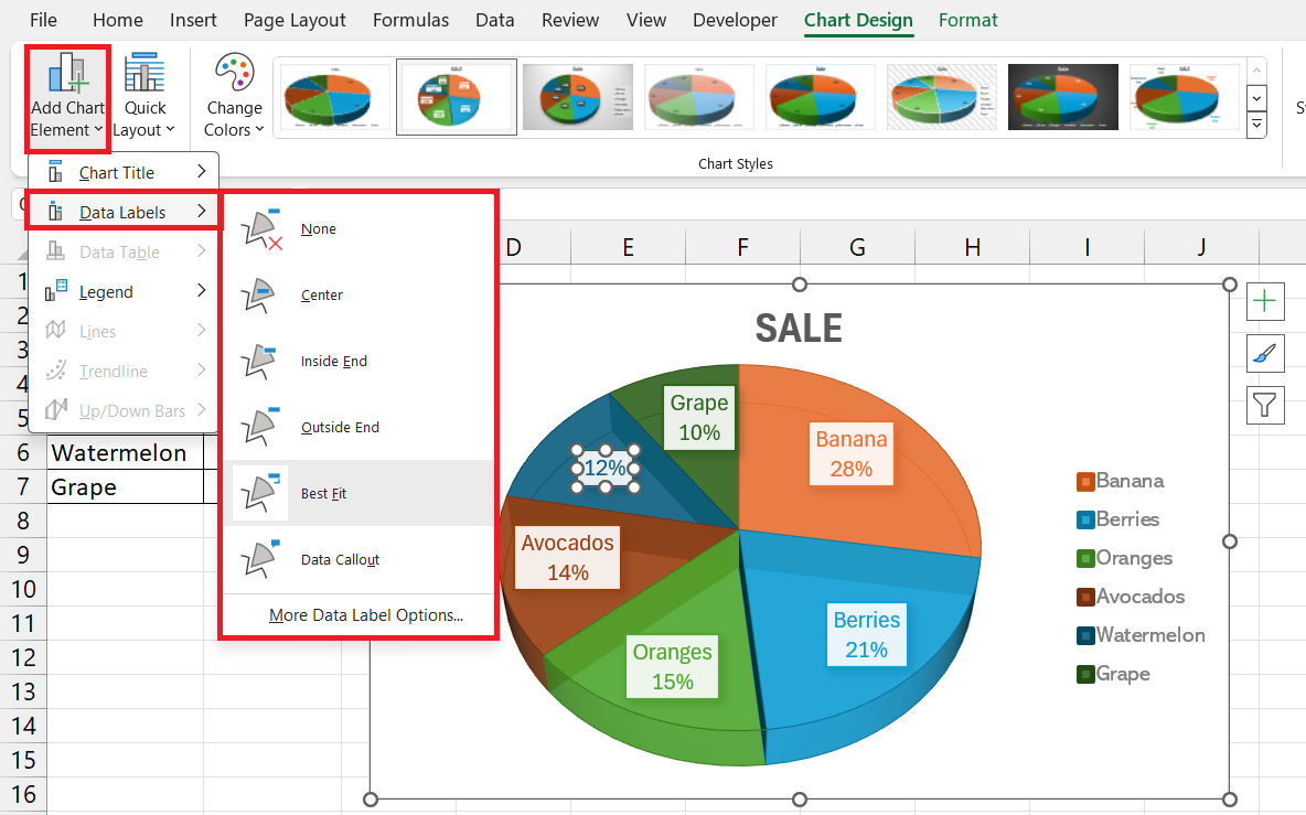
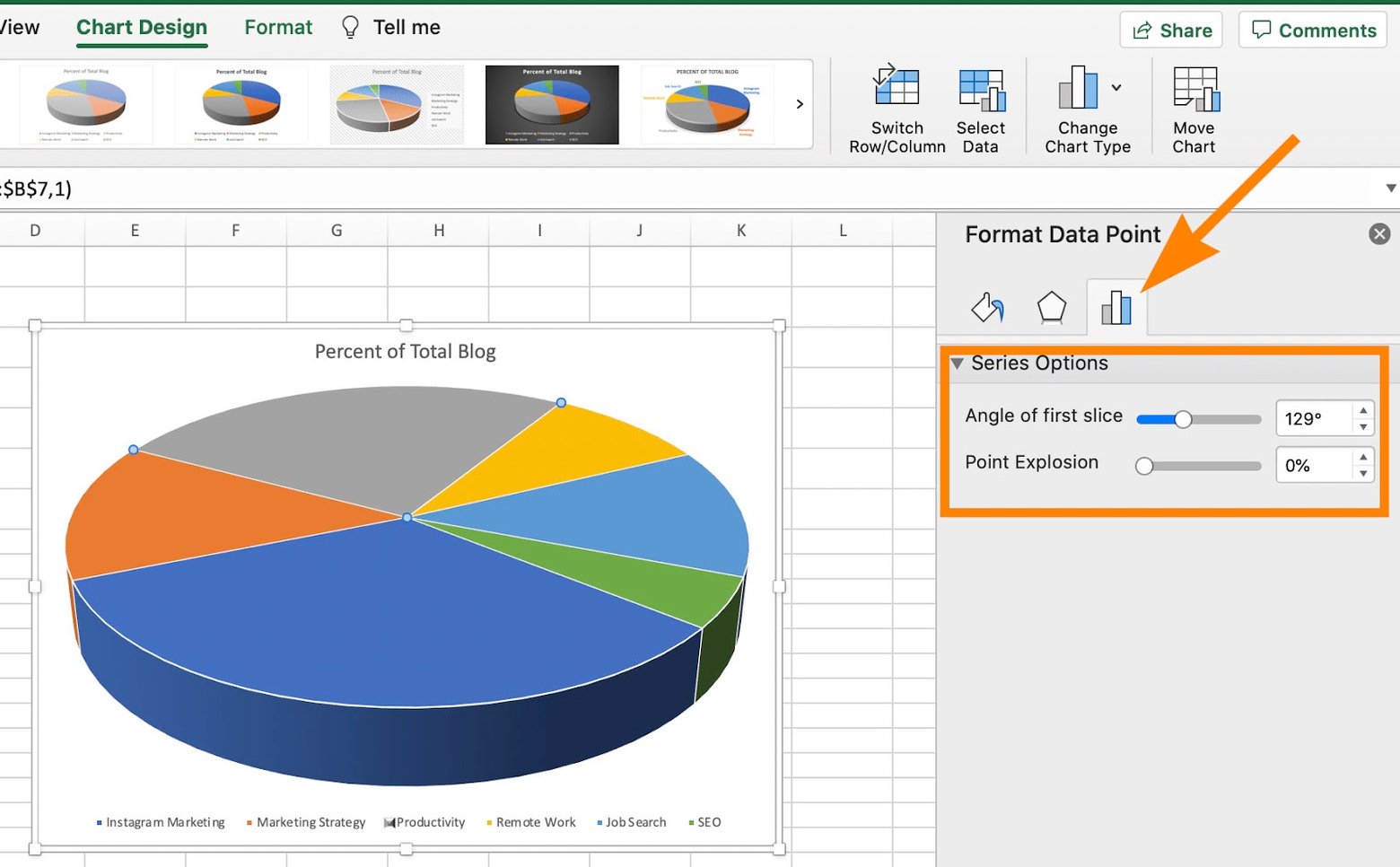
Create Pie Charts In Excel - How to create a pie chart in excel? To learn how to create and modify pie charts in excel, jump right into the guide below. A pie chart is a type of circular. We will use a sample dataset, which contains 2 columns: To quickly change the color. Go to the insert tab on the excel ribbon. Creating a pie chart in excel is easier than you might think! Download our free sample workbook here to tag along with the guide. In this article, we will show you how to create a pie of pie chart in excel, customize it, and use it for better data visualization in your spreadsheets. Click the pie chart icon. We have selected the range b4:c12. A pie chart is a type of circular. In this article, we will show you how to create a pie of pie chart in excel, customize it, and use it for better data visualization in your spreadsheets. How to create a pie chart in excel? An excel pie chart depicts the source data in. A pie chart is a type of circular. An excel pie chart depicts the source data in a circular graph. Pie charts always use one data series. To quickly change the color. To learn how to create and modify pie charts in excel, jump right into the guide below. We have selected the range b4:c12. A pie chart is a type of circular. Click the pie chart icon. Quick steps to add a pie chart prepare your chart data in microsoft excel select your data. Creating a pie chart in excel is easier than you might think! We will use a sample dataset, which contains 2 columns: In this article, we will show you how to create a pie of pie chart in excel, customize it, and use it for better data visualization in your spreadsheets. Pie charts are used to display the contribution of each value (slice) to a total (pie). We’ll show you how to. Click on the pie chart option within the charts group. A pie chart is a type of circular. An excel pie chart depicts the source data in a circular graph. Click the pie chart icon. Pie charts always use one data series. Download our free sample workbook here to tag along with the guide. To show, hide, or format things like axis titles or data labels, select chart elements. Pie charts always use one data series. To quickly change the color. Click on the pie chart option within the charts group. A pie chart is a type of circular. First, enter your data into an excel spreadsheet, select the data range, and then use the ‘insert’ tab to choose the. To show, hide, or format things like axis titles or data labels, select chart elements. To quickly change the color. Pie charts always use one data series. Go to the insert tab on the excel ribbon. First, enter your data into an excel spreadsheet, select the data range, and then use the ‘insert’ tab to choose the. To create a pie chart in excel, execute the following steps. In this article, we will show you how to create a pie of pie chart in excel, customize it,. To quickly change the color. We’ll show you how to create the chart, add category names, and. Pie charts always use one data series. Creating a pie chart in excel is easier than you might think! A pie chart is a type of circular. From the insert tab, select insert pie or. Download our free sample workbook here to tag along with the guide. First, enter your data into an excel spreadsheet, select the data range, and then use the ‘insert’ tab to choose the. Click the pie chart icon. We will use a sample dataset, which contains 2 columns: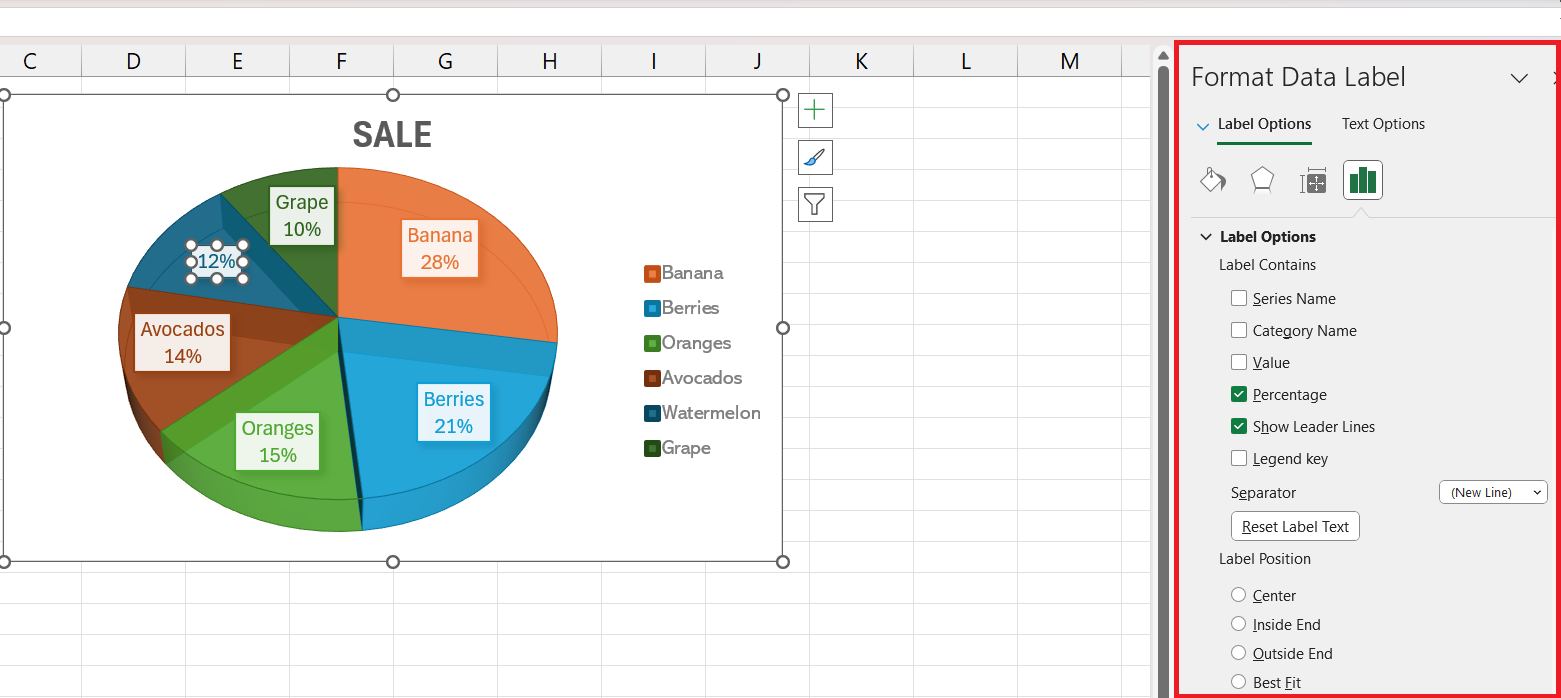
Create Pie Chart in Excel Like a Pro Fast & Simple Tutorial
:max_bytes(150000):strip_icc()/PieOfPie-5bd8ae0ec9e77c00520c8999.jpg)
Create An Excel Pie Chart Creating Pie Of Pie And Bar Of Pie
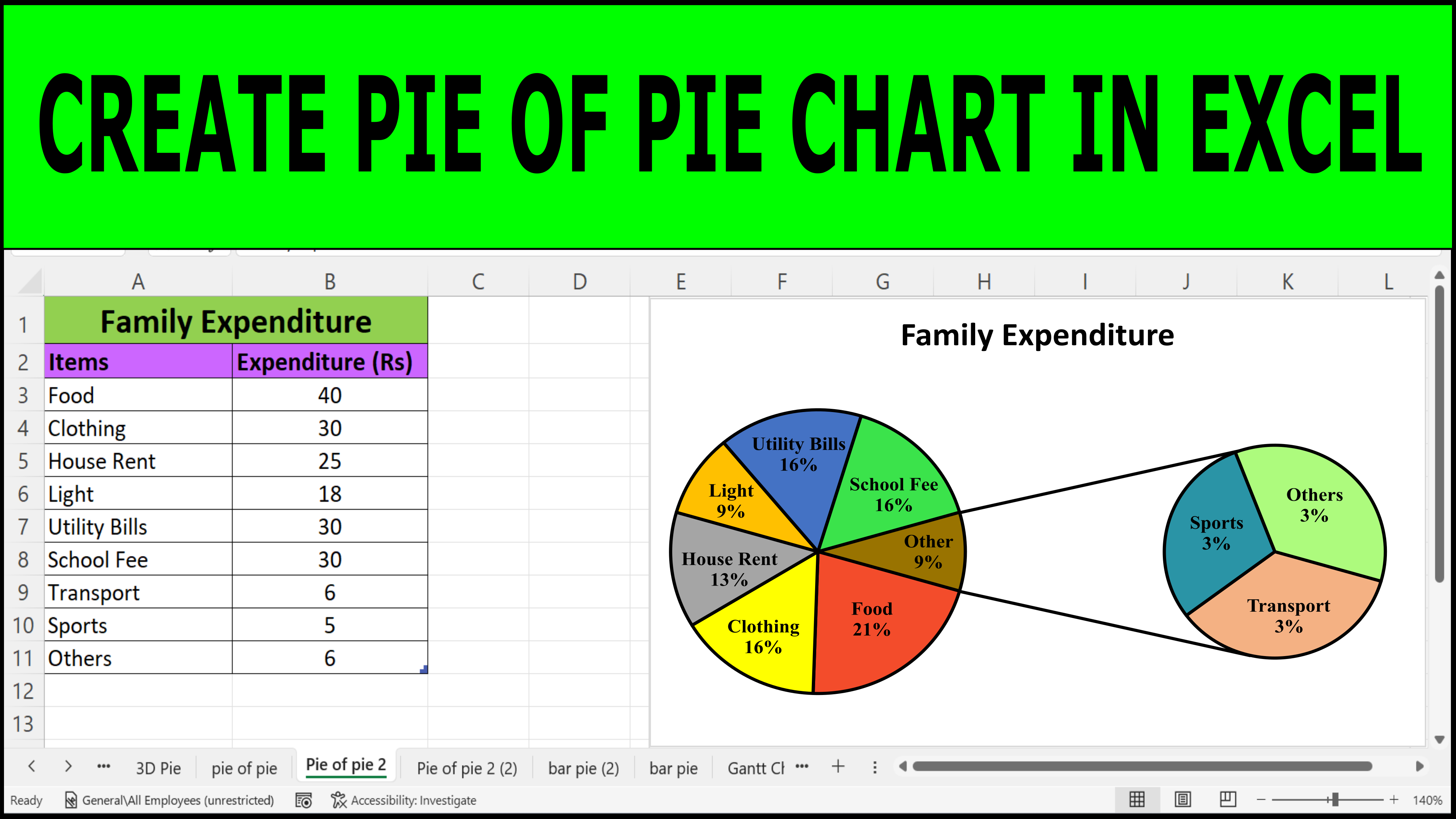
How to Create a Pie of Pie Chart in Excel
Create Pie Chart in Excel Like a Pro Fast & Simple Tutorial
Create Pie Chart in Excel Like a Pro Fast & Simple Tutorial
How To Create A Pie Chart In Excel (With Percentages) YouTube
Create pie chart in excel from data datelew
Create Pie Chart in Excel Like a Pro Fast & Simple Tutorial
How to Create a Pie Chart in Excel in 60 Seconds or Less
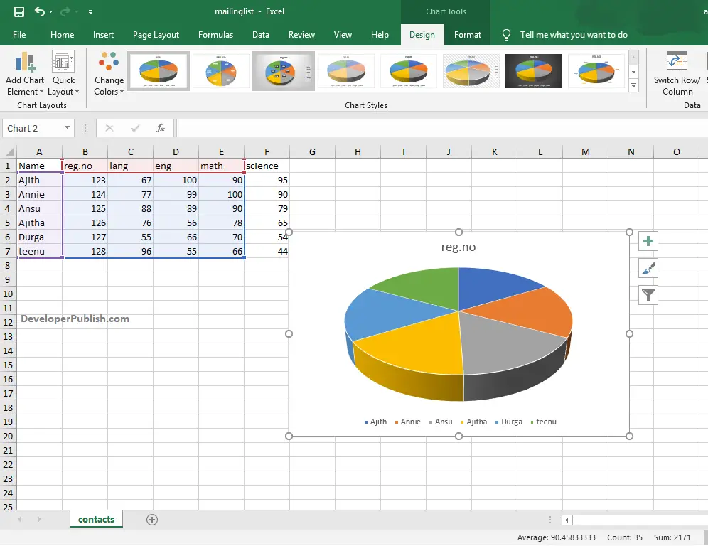
Pie Chart in Excel DeveloperPublish Excel Tutorials
Related Post: